Hamiltonian Monte Carlo
Implementation of the Hamiltonian Monte Carlo sampler for Bayesian inference.
-
HMC(U::Function, K::Function, dU::Function, dK::Function, init_est::Array{Float64}, d::Int64)¶ Construct a
Samplerobject for Hamiltonian Monte Carlo sampling.Arguments
U: the potential energy or the negative log posterior of the parameter of interest.K: the kinetic energy or the negative exponential term of the log auxiliary distribution.dU: the gradient or first derivative of the potential energyU.dK: the gradient or first derivative of the kinetic energyK.init_est: the initial/starting value for the markov chain.d: the dimension of the posterior distribution.
Value
Returns aHMCtype object.Example
In order to illustrate the modeling, the data is simulated from a simple linear regression expectation function. That is the model is given by
y_i = w_0 + w_1 x_i + e_i, e_i ~ N(0, 1 / a)
To do so, let
B = [w_0, w_1]' = [.2, -.9]', a = 1 / 5. Generate 200 hypothetical data:using DataFrames using Distributions using Gadfly using StochMCMC Gadfly.push_theme(:dark) srand(123); # Define data parameters w0 = -.3; w1 = -.5; stdev = 5.; a = 1 / stdev # Generate Hypothetical Data n = 200; x = rand(Uniform(-1, 1), n); A = [ones(length(x)) x]; B = [w0; w1]; f = A * B; y = f + rand(Normal(0, a), n); my_df = DataFrame(Independent = round(x, 4), Dependent = round(y, 4));
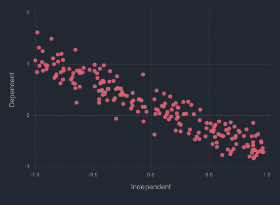
Next is to plot this data which can be done as follows:
plot(my_df, x = :Independent, y = :Dependent)
B ~ N(0, I), where 0 is the zero vector. The likelihood of the data is given by,L(w|[x, y], b) = ∏_{i=1}^n N([x_i, y_i]|w, b)Thus the posterior is given by,
P(w|[x, y]) ∝ P(w)L(w|[x, y], b)To start programming, define the probabilities
"""
The log prior function is given by the following codes:
"""
function logprior(theta::Array{Float64}; mu::Array{Float64} = zero_vec, s::Array{Float64} = eye_mat)
  w0_prior = log(pdf(Normal(mu[1, 1], s[1, 1]), theta[1]))
  w1_prior = log(pdf(Normal(mu[2, 1], s[2, 2]), theta[2]))
   w_prior = [w0_prior w1_prior]

  return w_prior |> sum
end

"""
The log likelihood function is given by the following codes:
"""
function loglike(theta::Array{Float64}; alpha::Float64 = a, x::Array{Float64} = x, y::Array{Float64} = y)
  yhat = theta[1] + theta[2] * x

  likhood = Float64[]
  for i in 1:length(yhat)
    push!(likhood, log(pdf(Normal(yhat[i], alpha), y[i])))
  end

  return likhood |> sum
end

"""
The log posterior function is given by the following codes:
"""
function logpost(theta::Array{Float64})
  loglike(theta, alpha = a, x = x, y = y) + logprior(theta, mu = zero_vec, s = eye_mat)
end
To start the estimation, define the necessary parameters
# Hyperparameters
zero_vec = zeros(2)
eye_mat = eye(2)
Setup the necessary paramters including the gradients. The potential energy is the negative logposterior given by
U, the gradient isdU; the kinetic energy is the standard Gaussian function given byK, with gradientdK. Thus,U(theta::Array{Float64}) = - logpost(theta); K(p::Array{Float64}; Σ = eye(length(p))) = (p' * inv(Σ) * p) / 2; function dU(theta::Array{Float64}; alpha::Float64 = a, b::Float64 = eye_mat[1, 1]) [-alpha * sum(y - (theta[1] + theta[2] * x)); -alpha * sum((y - (theta[1] + theta[2] * x)) .* x)] + b * theta end dK(p::AbstractArray{Float64}; Σ::Array{Float64} = eye(length(p))) = inv(Σ) * p;Run the MCMC:
srand(123);
HMC_object = HMC(U, K, dU, dK, zeros(2), 2);
chain2 = mcmc(HMC_object, leapfrog_params = Dict([:ɛ => .09, :τ => 20]), r = 10000);
Extract the estimate
est2 = mapslices(mean, chain2[(burn_in + 1):thinning:end, :], [1]);
est2
# 1×2 Array{Float64,2}:
#  -0.307151  -0.458954